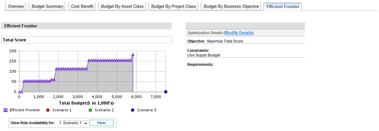
Understanding the Efficient Frontier Graph
As shown in the example in Figure 5-9. Scenario Comparison page, Efficient Frontier tab, the efficient frontier graph's horizontal axis is the budget and its vertical axis is one of the following performance objectives you chose to maximize:
-
NPV. NPV is the collective net present value for the lifecycle entities that the optimizer selects. For a definition of NPV, see Net Present Value (NPV).
-
Total Score. Total Score is the collective Total Score for the lifecycle entities that the optimizer selects. For information about how the Total Score for a lifecycle entity is calculated, see Determining Value and Risk Ratings.
-
Value. Value is the collective Value Rating for the lifecycle entities that the optimizer selects. For information about how the Value Rating for a lifecycle entity is calculated, see Determining Value and Risk Ratings.
The curve, calculated by the optimizer, is the efficient frontier—the best performance that can be achieved for your chosen objective when the optimal combinations (subsets) of all the lifecycle entities in this scenario comparison are used at various budget levels, within a set of constraints and requirements you specify (described later). The fewer such constraints and requirements, the higher the curve (that is, the better the performance) can be.
Note: To generate the efficient frontier, the scenario comparison must have a supply budget specified in the basic information (top section) of the scenario comparison.
The three scenarios of the scenario comparison being viewed provide three specific data points on the graph. The budget level (position on the horizontal axis) for a scenario data point is the sum of the costs for all the lifecycle entities in that scenario.
It is common for these scenario data points to fall below the efficient frontier curve. If you place no constraints on the optimizer's generation of the efficient frontier, the actual performance of any scenario, which specifies some particular combination of the lifecycle entities in this scenario comparison, will fall on or below the curve.
A scenario's data point can be above the curve, for either of the following reasons:
-
The constraints you specified in the efficient frontier parameters (as described in the procedure in Generating the Efficient Frontier Graph) are stricter than those of the scenario, so those constraints made the efficient frontier less successful than the scenario in meeting your objective at that supply budget level.
-
The efficient frontier curve has not been regenerated since the scenario was changed in such a way that the scenario's performance improved.
Note: You can invoke the optimizer for any of the scenarios in a scenario comparison, to determine the best subset of all the lifecycle entities in the scenario comparison to use for your performance objective. See Running Scenario Optimizations. (Running a scenario optimization does not generate the efficient frontier curve.) If you use the same set of constraints to both optimize a scenario and generate the efficient frontier, that scenario's data point will fall on the efficient frontier curve.
The right side of the Efficient Frontier tab displays the objective, the budget and resource constraints, and any other requirements that were specified in the first Efficient Frontier window when the curve was last generated (see Generating the Efficient Frontier Graph).


